Diffusion Models
约 3098 个字 9 张图片 预计阅读时间 10 分钟
Abstract
这一节的内容我先看了CS236的部分,Stefano对Diffusion的讲解主要建立在Score-based Models的基础上,这也是一种理解扩散模型的视角,然后我看了MIT的6.S184对于这部分的讲解。但我觉得最有帮助的部分还是lilian weng的博客,及其严谨的推导和连贯的思路,我的博客榜样!()
Intro
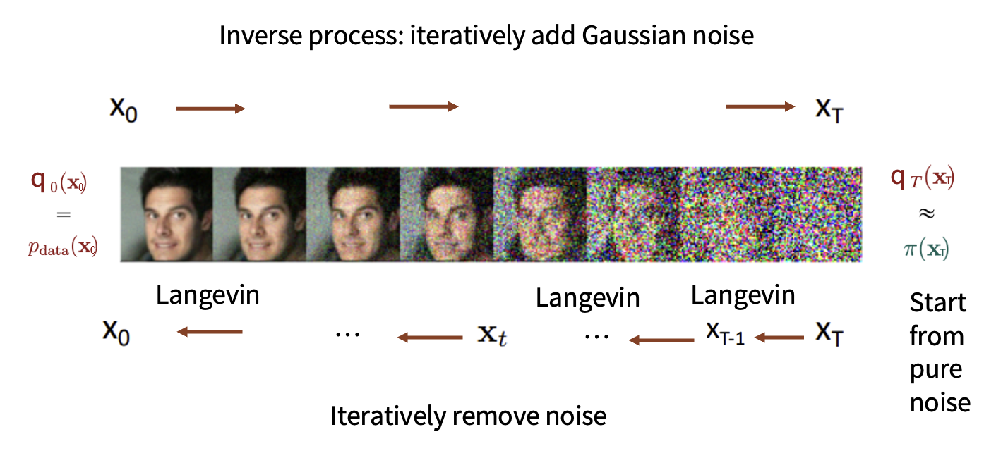
回顾一下我们在Score-based Models中介绍的分数模型方法,我们定义一个分数来对数据分布进行评价,在denoising score matching中,通过加噪过程,得到一个易于采样的数据,再通过去噪过程,得到一个去噪后的数据,这个去噪后的数据就是我们的目标数据。
在Diffusion Models中,我们也做了类似的事情:
接下来的工作就是看如何重新定义这个马尔可夫过程的细节,具体到计算层面。
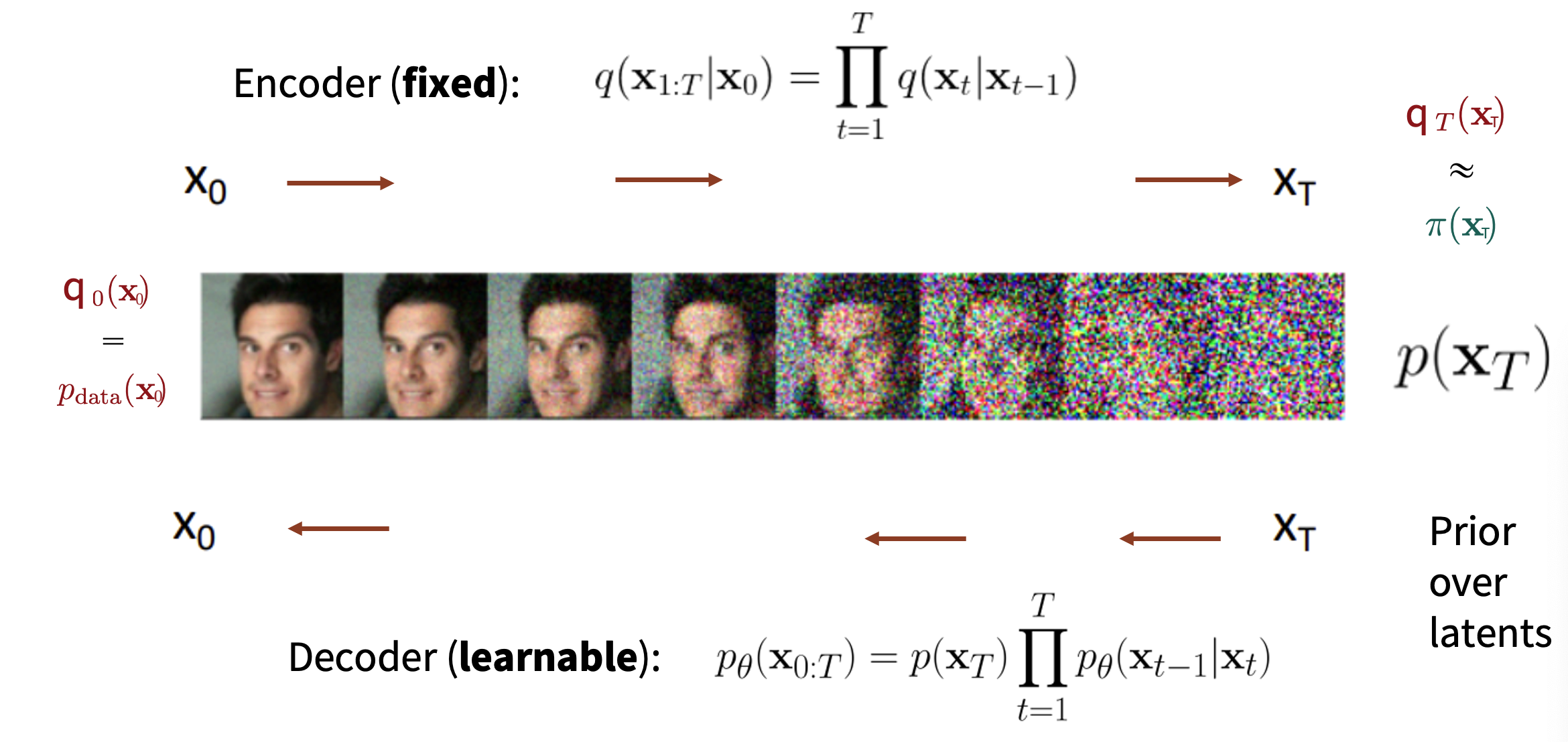
Noising Process
这里基本上与denoising score matching类似
同时这一步骤也可以采用multi-step的方式,即:
其中,\(\bar{\alpha}_t = \prod_{i=1}^t (1-\beta_i)\)。
Diffusion Process
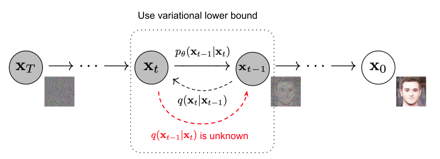
按照思路进行下去,我们在逆向过程中只需要做 iteratively sample from \(q(x_{t-1}|x_t)\),但问题是:
这个真实计算量非常大(用贝叶斯定理展开发现我们需要计算t-1和t时刻的边缘概率分布,这需要对前面的所有时刻进行积分)
我们的解决措施是学一个变分近似\(p_\theta(x_{t-1}|x_t)\)来对真实分布进行近似
为什么这样近似?
虽然\(q(x_{t-1}|x_t)\)是未知的,但通过数学推导我们可以证明,在给定了先验\(x_0\)的情况下,\(q(x_{t-1}|x_t, x_0)\)会变成一个可计算的高斯分布,他的方差和均值都可以用给定的\(\beta_t\)来得到
证明
卧槽好多公式
我们的目标是证明\(q(x_{t-1}|x_t, x_0)\)是一个高斯分布,并且他的方差和均值都可以用给定的\(\beta_t\)来得到
用贝叶斯展开这个式子:
由马尔可夫过程的性质,我们知道\(x_t\)只与\(x_{t-1}\)有关,与\(x_0\)无关,所以\(q(x_t|x_{t-1}, x_0) = q(x_t|x_{t-1})\),同时\(q(x_t|x_0)\)与\(x_{t-1}\)无关,所以分母当作常数我们不看
这样此时目标正比于这两个部分:
因为一个正态分布的pdf的指数上满足:\(\exp(-\frac{(x-\mu)^2}{2\sigma^2}) = \exp(-\frac{x^2}{2\sigma^2} + \frac{x\mu}{\sigma^2} - \frac{\mu^2}{2\sigma^2})\),所以我们知道只需要得到二次项和一次项系数,就可以知道这个分布的均值和方差
展开后我们得到指数部分为:
所以此时我们能得到方差和均值:
成功证明:\(q(x_{t-1}|x_t, x_0) \sim \mathcal{N}(x_{t-1}; \tilde\mu_t, \tilde\beta_t\mathbf{I})\)
并且也可以显然看出,他们都是关于给定参数的可计算函数
所以这启发我们,我们只需要学习一个神经网络来近似\(\tilde\mu_t\)和\(\tilde\beta_t\),就可以得到一个变分近似\(p_\theta(x_{t-1}|x_t)\)(在实际情况(比如DDPM)中,我们只需要学习\(\tilde\mu_t\)):
进而得到最终的joint distribution,也就是我们的结果:
课上Stefano说经过证明,如果我们做的是朗之万采样,这里的\(\mu_\theta\)甚至就是sm中的score(wtf?)原因之后会说到。
Training
到目前为止,我们已经得到了两个模块,encoder & decoder
现在我们需要讨论一下training的问题
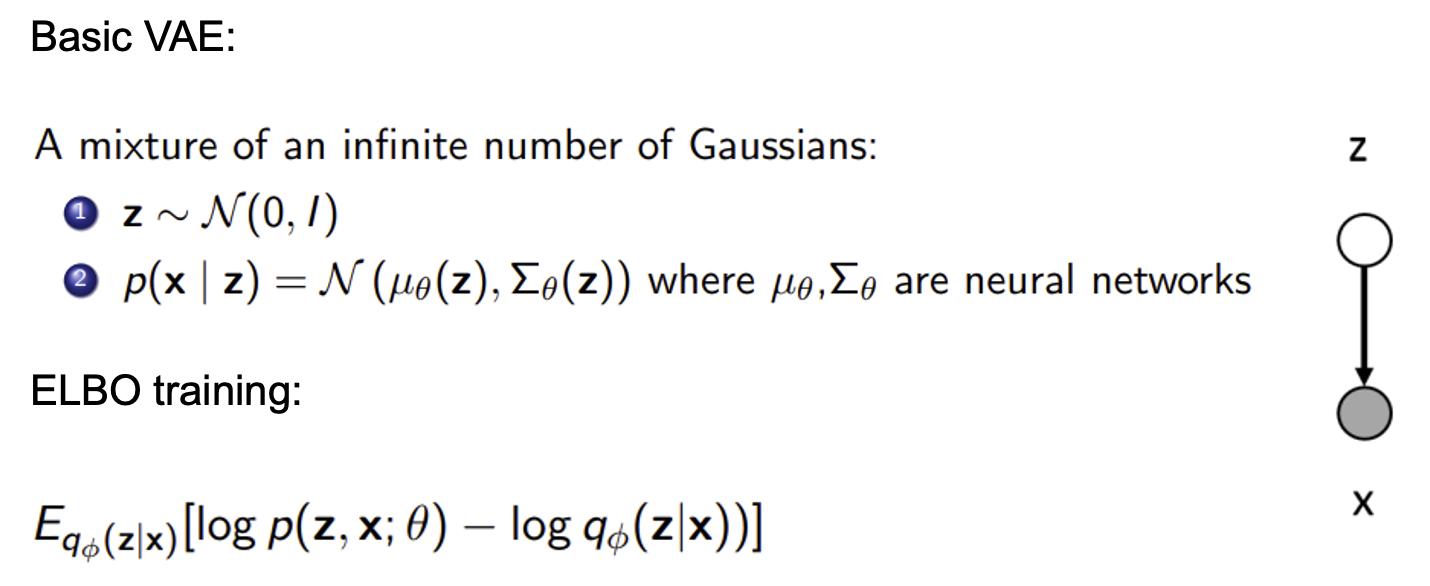
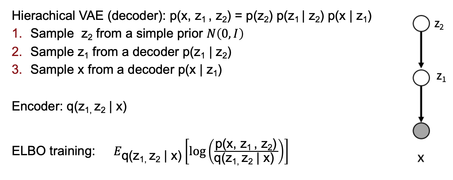
如果只对Diffusion过程的一步进行观察,我们发现这一过程很像是VAE对隐变量解码的过程:
所以我们使用与ELBO类似的变分下界来进行训练
最原始的VAE loss是:
然后我们看增加latent层数后:
按照这个思路,我们可以得到层数为T的Diffusion Models的loss:
Loss of Diffusion Models
推导
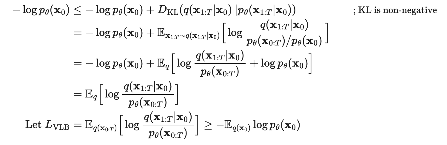
但是现在得到的这个loss是很难计算的,所以需要进行computable转换:
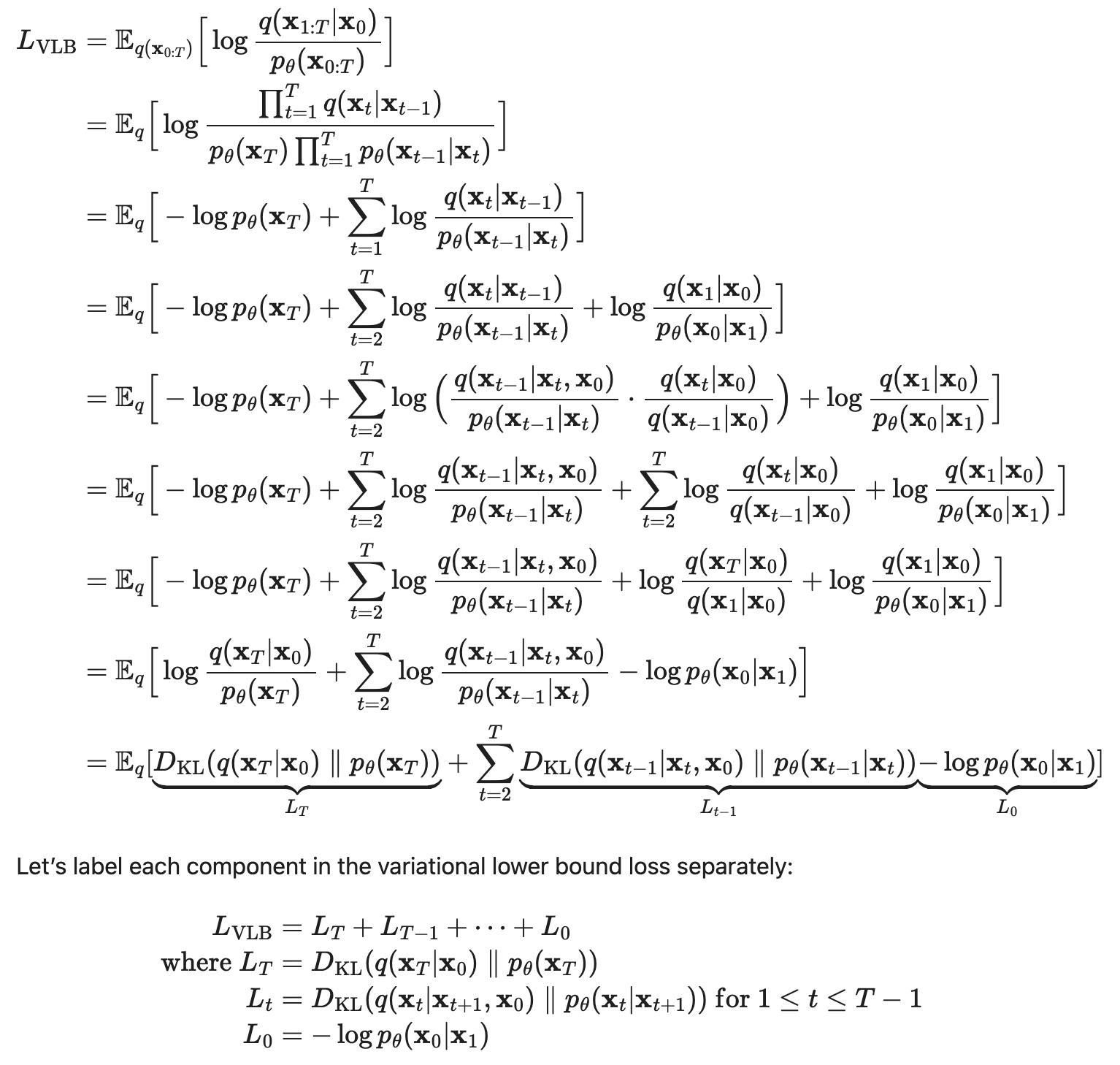
现在我们得到的这三种L中\(L_0\)是常量,而\(L_T\)中的\(x_T\)是已知的,我们忽略掉最后一项,将第一项设置为高斯分布
现在需要处理\(L_t\),对其进行参数化:
- 对\(\mu_\theta\)进行参数化,因为在每一步我们是知道\(x_t\)的,所以就是对噪声\(\epsilon_t\)进行参数化,这时的Loss被参数化为minimize \(\mu_\theta\) 和 \(\tilde \mu_t\),并最终化简为:
推导
这里lilian的博客中直接给出了带入近似的\(\mu_\theta\)的结果,我来稍微推导一下,主要是利用了KL在计算两个高斯分布时的性质,即:
其中d是维度,因为在DDPM中方差被固定不学习了,模型与真实分布方差相等后,上式就被简化:
这时我们再带入\(\mu_\theta\)和\(\tilde\mu_t\)即可
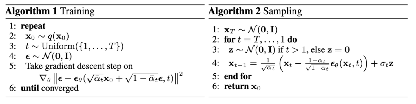
在实际的操作中,DDPM发现训练目标可以进行化简,放弃噪声距离前的那个权重,所以最终我们的loss被简化为:
至此,我们就推导出了Diffusion Models原文算法中的各项内容:
Relation to Score Matching
我想Score-based Models的思路这里可以不再做重复了,我们来看一下核心的部分,也就是score function,为了对比,我在这里使用ddpm中的notation:
由于我们使用的是高斯分布:
推导过程(Gemini)
证明 \(\nabla_{\mathbf{x}_t} \log q(\mathbf{x}_t) = \mathbb{E}_{q(\mathbf{x}_0|\mathbf{x}_t)}[\nabla_{\mathbf{x}_t} \log q(\mathbf{x}_t|\mathbf{x}_0)]\)
-
从左侧 (LHS) 出发
我们从等式左侧的定义开始,应用对数求导法则 \(\nabla \log f(x) = \frac{\nabla f(x)}{f(x)}\):
\[\nabla_{\mathbf{x}_t} \log q(\mathbf{x}_t) = \frac{\nabla_{\mathbf{x}_t} q(\mathbf{x}_t)}{q(\mathbf{x}_t)}\] -
展开边缘概率 \(q(\mathbf{x}_t)\)
\(q(\mathbf{x}_t)\) 是带噪数据的边缘概率分布。它是通过将联合分布 \(q(\mathbf{x}_t, \mathbf{x}_0)\) 对所有可能的初始数据 \(\mathbf{x}_0\) 进行积分得到的。而联合分布可以写作 \(q(\mathbf{x}_t, \mathbf{x}_0) = q(\mathbf{x}_t|\mathbf{x}_0)p_{data}(\mathbf{x}_0)\)。
\[q(\mathbf{x}_t) = \int q(\mathbf{x}_t|\mathbf{x}_0) p_{data}(\mathbf{x}_0) d\mathbf{x}_0\]现在我们对它求梯度。梯度算子 \(\nabla_{\mathbf{x}_t}\) 可以移动到积分号内部(在满足一定正则性条件下,此处成立):
\[\nabla_{\mathbf{x}_t} q(\mathbf{x}_t) = \int \nabla_{\mathbf{x}_t} q(\mathbf{x}_t|\mathbf{x}_0) p_{data}(\mathbf{x}_0) d\mathbf{x}_0\] -
再次使用对数求导法则(逆向)
注意到 \(\nabla f(x) = f(x) \nabla \log f(x)\),我们可以将这个技巧应用到积分号内部的项 \(\nabla_{\mathbf{x}_t} q(\mathbf{x}_t|\mathbf{x}_0)\) 上:
\[\nabla_{\mathbf{x}_t} q(\mathbf{x}_t|\mathbf{x}_0) = q(\mathbf{x}_t|\mathbf{x}_0) \nabla_{\mathbf{x}_t} \log q(\mathbf{x}_t|\mathbf{x}_0)\]将这个结果代回到第2步的梯度表达式中:
\[\nabla_{\mathbf{x}_t} q(\mathbf{x}_t) = \int q(\mathbf{x}_t|\mathbf{x}_0) \nabla_{\mathbf{x}_t} \log q(\mathbf{x}_t|\mathbf{x}_0) p_{data}(\mathbf{x}_0) d\mathbf{x}_0\] -
识别出期望的形式
现在我们把第3步的结果代回到第1步的LHS表达式中:
\[\nabla_{\mathbf{x}_t} \log q(\mathbf{x}_t) = \frac{\int q(\mathbf{x}_t|\mathbf{x}_0) \nabla_{\mathbf{x}_t} \log q(\mathbf{x}_t|\mathbf{x}_0) p_{data}(\mathbf{x}_0) d\mathbf{x}_0}{q(\mathbf{x}_t)}\]现在,我们对分子中的 \(q(\mathbf{x}_t|\mathbf{x}_0) p_{data}(\mathbf{x}_0)\) 应用贝叶斯定理,它等于 \(q(\mathbf{x}_0|\mathbf{x}_t)q(\mathbf{x}_t)\):
\[\nabla_{\mathbf{x}_t} \log q(\mathbf{x}_t) = \frac{\int \nabla_{\mathbf{x}_t} \log q(\mathbf{x}_t|\mathbf{x}_0) \cdot q(\mathbf{x}_0|\mathbf{x}_t) q(\mathbf{x}_t) d\mathbf{x}_0}{q(\mathbf{x}_t)}\]由于积分是关于 \(\mathbf{x}_0\) 的,\(q(\mathbf{x}_t)\) 可以被看作常数从积分中提出来:
\[\nabla_{\mathbf{x}_t} \log q(\mathbf{x}_t) = \frac{q(\mathbf{x}_t) \int \nabla_{\mathbf{x}_t} \log q(\mathbf{x}_t|\mathbf{x}_0) q(\mathbf{x}_0|\mathbf{x}_t) d\mathbf{x}_0}{q(\mathbf{x}_t)}\]上下消去 \(q(\mathbf{x}_t)\):
\[\nabla_{\mathbf{x}_t} \log q(\mathbf{x}_t) = \int \nabla_{\mathbf{x}_t} \log q(\mathbf{x}_t|\mathbf{x}_0) q(\mathbf{x}_0|\mathbf{x}_t) d\mathbf{x}_0\]这个最后的积分形式,正是期望的定义。它表示的是函数 \(\nabla_{\mathbf{x}_t} \log q(\mathbf{x}_t|\mathbf{x}_0)\) 在概率分布 \(q(\mathbf{x}_0|\mathbf{x}_t)\) 下的期望值。所以:
\[\nabla_{\mathbf{x}_t} \log q(\mathbf{x}_t) = \mathbb{E}_{q(\mathbf{x}_0|\mathbf{x}_t)}[\nabla_{\mathbf{x}_t} \log q(\mathbf{x}_t|\mathbf{x}_0)]\]至此,我们证明了等式成立。
可以看到score所在的位置就是sampling中\(x_t\)的更新方向
Conditional Diffusion Models
在给定约束(label)的情况下,我们如何训练Diffusion Models?有以下两种思路:
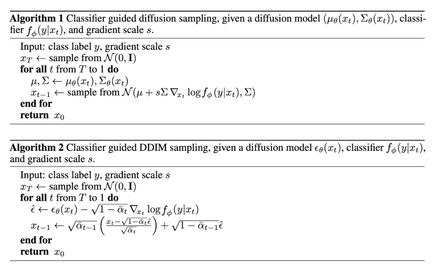
Classifier Guided Diffusion
将类别信息显式地加入到score中,对联合分布\(q(\mathbf{x}_t, y)\)进行优化
这时新的predictor就是:
其中w用于控制分类强度
Classifier-Free Diffusion Guidance
Efficient Diffusion Models
留言